Executing gradient descent on the planet

Executing gradient descent on the planet

September 19, 2017 — Chris Foster

A accepted analogy for explaining gradient descent goes admire the following: an particular individual is caught in the mountains throughout heavy fog, and ought to navigate their come down. The pure come they’ll come this is to be taught about at the slope of the visible floor spherical them and slowly work their come down the mountain by following the downward slope.

This captures the essence of gradient descent, however this analogy always ends up breaking down after we scale to a high dimensional house where we have very runt device what the right kind geometry of that house is. Despite the undeniable truth that, in the close it’s assuredly no longer an even wretchedness because gradient descent appears to work relatively grand.

But the well-known question is: how neatly does gradient descent originate on the right kind earth?

Defining a be aware feature and weights

In a overall mannequin gradient descent is aged to construct up weights for a mannequin that minimizes our be aware feature, which is on the entire some representation of the errors made by a mannequin over quite a lot of predictions. We don’t beget a mannequin predicting the leisure in this case and attributable to this truth no “errors”, so adapting this to touring spherical the earth requires some stretching of the stylish machine studying context.

In our earth-streak touring algorithm, our goal goes to be to construct up sea level from wherever our starting cases are. That is, we can account for our “weights” to be a latitude and longitude and we can account for our “be aware feature” to be the sleek high from sea level. Put one more come, we are asking gradient descent to optimize our latitude and longitude values such that the head from sea level is minimized. Unfortunately, we don’t beget a mathematical feature that describes the full earth’s geography so we can calculate our be aware values the employ of a raster elevation dataset available from NASA:

import rasterio

# Delivery the elevation dataset
src = rasterio.start(sys.argv[1])
band = src.read(1)

# Procure the elevation
def get_elevation(lat, lon):
    vals = src.index(lon, lat)
    return band[vals]

# Calculate our 'be aware feature'
def compute_cost(theta):
    lat, lon = theta[0], theta[1]
    J = get_elevation(lat, lon)
    return J

Gradient descent works by having a be taught about at the gradient of the rate feature with respect to every variable it’s optimizing for, and adjusting the variables such that they originate a decrease be aware feature. Right here’s easy when your be aware feature is a mathematical metric admire imply squared error, however as we mentioned our “be aware feature” is a database search for so there isn’t the leisure to safe the spinoff of.

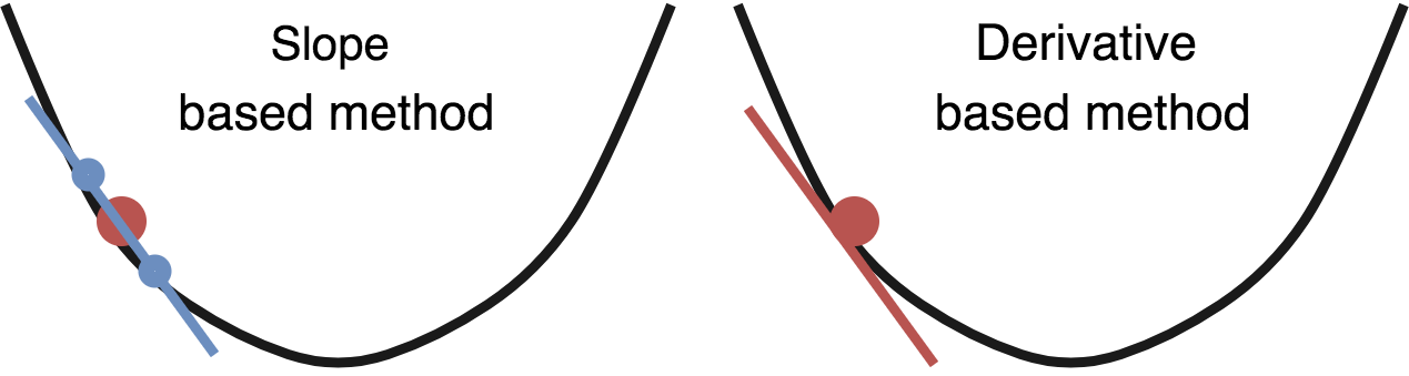
Fortunately, we can approximate the gradient the identical come our human explorer in our analogy would: by having a be taught about spherical. The gradient is identical to the slope, so we can estimate the slope by taking some extent a runt bit above our sleek space and some extent honest under it (in each and every dimension) and divide them to safe our estimated spinoff. This ought to work reasonably neatly:

def gradient_descent(theta, alpha, gamma, num_iters):
    J_history = np.zeros(shape=(num_iters, 3))
    velocity = [ 0, 0 ]

    for i in fluctuate(num_iters):

        be aware = compute_cost(theta)

        # Procure elevations at offsets in each and every dimension
        elev1 = get_elevation(theta[0] + 0.001, theta[1])
        elev2 = get_elevation(theta[0] - 0.001, theta[1])
        elev3 = get_elevation(theta[0], theta[1] + 0.001)
        elev4 = get_elevation(theta[0], theta[1] - 0.001)

        J_history[i] = [ be aware, theta[0], theta[1] ]
        if be aware <= 0: return theta, J_history

        # Calculate slope
        lat_slope = elev1 / elev2 - 1
        lon_slope = elev3 / elev4 - 1 

        # Replace variables
        theta[0][0] = theta[0][0] - lat_slope
        theta[1][0] = theta[1][0] - lon_slope

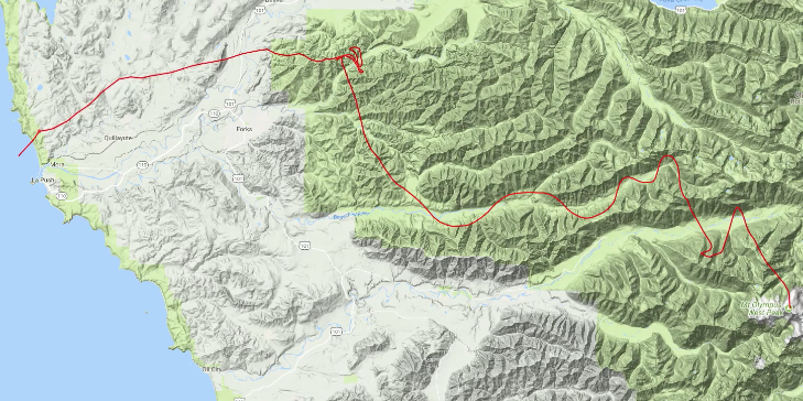
    return theta, J_history

Tall! You’ll sight that this differs from most implementations of gradient descent in that there is now not any longer a X or y variables passed into this selection. Our be aware feature doesn’t require calculating the error of any predictions, so we handiest need the variables we are optimizing here. Let’s strive working this on Mount Olympus in Washington:

Hm, it appears to safe caught! This happens testing in most other areas as neatly. It turns out that the earth is stuffed with native minima, and gradient descent has a enormous amount of wretchedness discovering the area minimal when starting in a local house that’s even a runt bit some distance from the ocean.

Momentum optimization

Vanilla gradient descent isn’t our handiest software program in the box, so we can strive momentum optimization. Momentum is electrified by proper physics, which makes the utility of it to gradient descent on proper geometry a elegant device. Unfortunately, if we assign even an extraordinarily right bolder at the head of Mount Olympus and let it dash, it’s no longer going to beget ample momentum to realize the ocean, so we’ll need to employ some unrealistic (in physical phrases) values of gamma here:

def gradient_descent(theta, alpha, gamma, num_iters):
    J_history = np.zeros(shape=(num_iters, 3))
    velocity = [ 0, 0 ]

    for i in fluctuate(num_iters):

        be aware = compute_cost(theta)

        # Procure elevations at offsets in each and every dimension
        elev1 = get_elevation(theta[0] + 0.001, theta[1])
        elev2 = get_elevation(theta[0] - 0.001, theta[1])
        elev3 = get_elevation(theta[0], theta[1] + 0.001)
        elev4 = get_elevation(theta[0], theta[1] - 0.001)

        J_history[i] = [ be aware, theta[0], theta[1] ]
        if be aware <= 0: return theta, J_history

        # Calculate slope
        lat_slope = elev1 / elev2 - 1
        lon_slope = elev3 / elev4 - 1 

        # Calculate replace with momentum
        velocity[0] = gamma * velocity[0] + alpha * lat_slope
        velocity[1] = gamma * velocity[1] + alpha * lon_slope

        # Replace variables
        theta[0][0] = theta[0][0] - velocity[0]
        theta[1][0] = theta[1][0] - velocity[1]

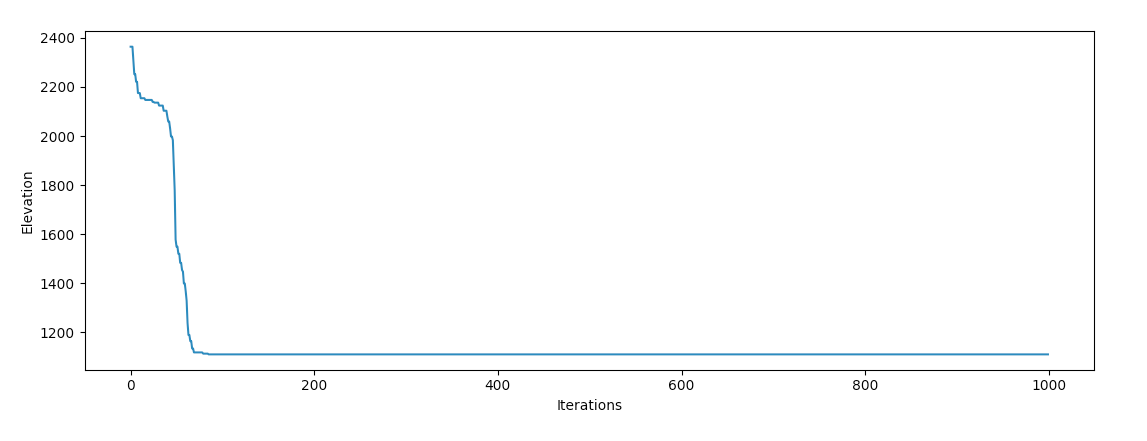
    return theta, J_history

With some variable tweaking, gradient descent will need to beget a more in-depth likelihood of discovering the ocean:

We’ve got success! It’s inviting gazing the behaviour of the optimizer, it appears to tumble into a valley and “roll off” each and every of the perimeters on it’s come down the mountain, which agrees with our intuition of how an object with extraordinarily high momentum ought to behave bodily.

Closing options

The earth ought to in reality be a very easy feature to optimize. For the reason that earth is essentially lined by oceans, more than two thirds of likely legitimate inputs for this selection return the optimal be aware feature worth. Nonetheless, the earth is plagued with native minima and non-convex geography.

Thanks to this, I own it provides rather about a inviting alternatives for exploring how machine studying optimization methods originate on tangible and understandable native geometries. It appears to originate relatively grand on Mount Olympus, so let’s name this analogy “confirmed”!

In case you are going to need got options on this, let me know on twitter!

The code for the venture is available here.