Compressing and making improvements to hand-written notes

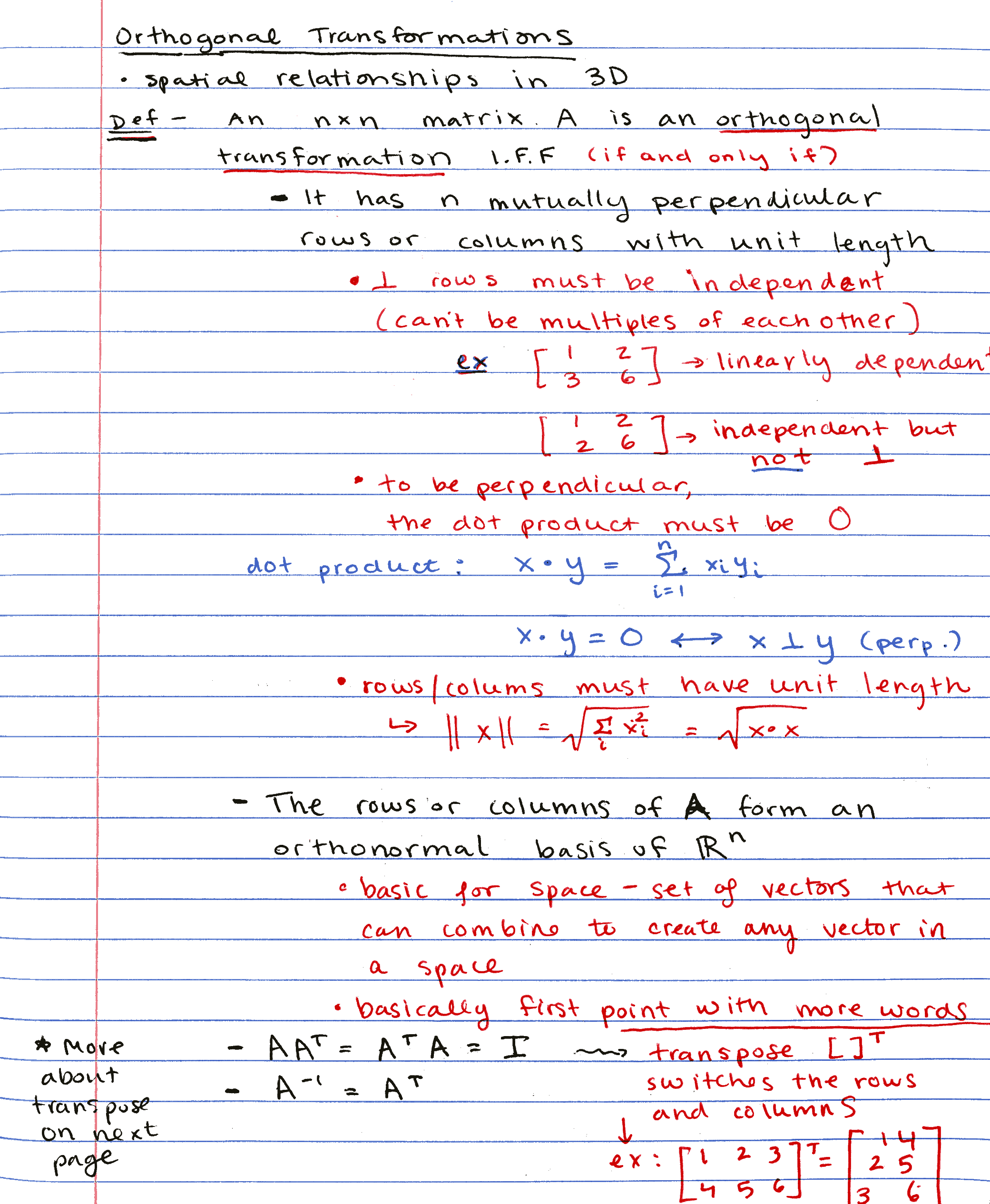
I wrote a program to dapper up scans of handwritten notes whereas concurrently reducing file size.

Instance enter and output:

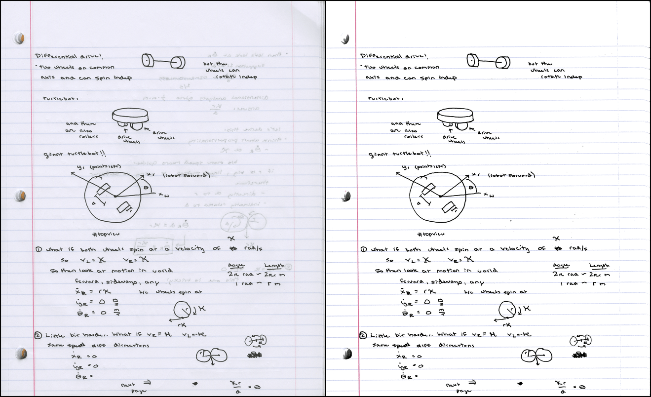
Left: enter scan @ 300 DPI, 7.2MB PNG / 790KB JPG. Upright:
output @ identical resolution, 121KB PNG.

Disclaimer: the technique described here is roughly what the
Position of job Lens app does already, and there’s maybe any number of
other tools that attain equivalent things. I’m no longer claiming to have come up
with a thorough unusual invention – true my hang implementation of a worthwhile
instrument.

If you occur to’re in a speed, true take a look at out the github repo, or jump down
to the results part, where you are going to have the choice to play with
interactive 3D diagrams of color clusters.

About a of my classes don’t have an assigned textbook. For these, I hang
to nominate weekly “student scribes” to part their lecture notes with
the reduction of the category, so that there’s some form written resource for
college students to double-take a look at their notion of the topic fabric. The
notes earn posted to a route web situation as PDFs.

In college we have got a “pleasing” copier good of scanning to PDF, but the
documents it produces are… no longer as a lot as beautiful. Here’s some instance
output from a handwritten homework page:

Seemingly at random, the copier chooses whether to binarize each and every
label (hang the x’s), or turn them into abysmally blocky JPGs (hang
the square root symbols). Pointless to converse, we can attain better.

We commence out with a scan of a handsome page of student notes hang this one:

The traditional PNG image scanned at 300 DPI is about 7.2MB; the equivalent
image remodeled to a JPG at quality stage 85 is about 790KB. Since
PDFs of scans are in general true a container layout round PNG
or JPG, we undoubtedly don’t build an tell to to lower the main storage
size when converting to PDF. 800KB per page is barely hefty – for the
sake of loading instances, I’d gain to be aware things closer to
100KB/page.

Even supposing this student is a extraordinarily tidy lisp-taker, the scan confirmed above
looks rather messy (through no fault of her hang). There’s a entire bunch
bleed-through from the opposite aspect of the page, which is both
distracting for the viewer and exhausting for a JPG or PNG encoder to
compress, when put next to a fixed-color background.

Here’s what the output of my noteshrink.py program looks hang:

It’s a relatively cramped PNG file, weighing in at true 121KB. My
current part? No longer simplest did the image earn smaller, it also obtained
clearer!

Here are the steps required to contrivance the compact, dapper image above:

1. Name the background color of the traditional scanned image.

2. Isolate the foreground by thresholding on distinction from background color.

3. Convert to an indexed color PNG by picking a tiny number of
   “representative colours” from the foreground.

Ahead of we delve into each and every of these steps, it’ll be worthwhile to
recap how color pictures are saved digitally. Because folk have
three various kinds of color-tender cells of their eyes, we can
reconstruct any color by combining various intensities of crimson, inexperienced,
and blue light. The resulting system equates colours with 3D
parts in the RGB colorspace, illustrated here:

Even supposing an even vector dwelling would enable an unlimited number of
repeatedly various pixel intensities, we have got to discretize colours
in lisp to store them digitally – in general assigning eight bits each and every to
the crimson, inexperienced, and blue channels. Alternatively, pondering colours
in an image analogously to parts in a continuous 3D dwelling offers
noteworthy tools for diagnosis, as we shall seek after we step during the
route of outlined above.

For the rationale that majority of the page is free from ink or lines, we might maybe
build an tell to the paper color to be the one who looks most frequently in
the scanned image – and if the scanner continuously represented each and every bit
of unmarked white paper because the equivalent RGB triplet, we would wouldn’t have any
complications picking it out. Regrettably, here is no longer the case; random
diversifications in color appear due to this of dirt specks and smudges on the
glass, color diversifications of the page itself, sensor noise, and so forth. So in
reality, the “page color” can spread all over 1000’s of determined
RGB values.

The traditional scanned image is 2,081 x 2,531, with a entire exclaim of
5,267,011 pixels. Even supposing we might maybe preserve in thoughts each and every particular person pixel,
it’s valuable faster to work on a representative sample of the enter
image. The noteshrink.py program samples 5% of the enter image by
default (extra than ample for scans at 300 DPI), but for now,
let’s take a study an very obedient smaller subset of 10,000 pixels chosen at random
from the traditional scan:

Even supposing it bears scant resemblance to the true scanned page –
there’s no textual declare to be stumbled on – the distribution of colours in the two
pictures is barely valuable equivalent. Both are mostly grayish-white, with a
handful of crimson, blue, and sad grey pixels. Here are the equivalent 10,000
pixels, sorted by brightness (e.g. the sum of their R, G, and B
intensities):

Considered from afar, the bottom eighty-Ninety% of the image all looks to be the
identical color; alternatively, closer inspection unearths rather rather of variation.
In spite of the entire lot, essentially the most frequent color in the image above, with RGB worth
(240, 240, 242), accounts for true 226 of the ten,000 samples – less
than Three% of the overall number of pixels.

Because the mode here accounts for this kind of tiny proportion of the
sample, we ought to ask how reliably it describes the distribution
of colours in the image. We’ll have the next likelihood of figuring out a
prevalent page color if we first lower the bit depth of the image
sooner than discovering the mode. Here’s what things look hang after we switch
from eight bits per channel to 4 by zeroing out the 4
least main bits:

Now essentially the most frequently occurring color has RGB worth (224, 224, 224),
and accounts for Three,623 (36%) of the sampled pixels. Essentially, by
reducing the bit depth, we’re grouping equivalent pixels into greater
“boxes”, which makes it more uncomplicated to win a solid peak in the suggestions.

There’s a tradeoff here between reliability and precision: tiny boxes
enable finer distinctions of color, but bigger boxes are valuable extra
sturdy. Within the tip, I went with 6 bits per channel to title the
background color, which looked hang an even candy location between the two
extremes.

As soon as we have got identified the background color, we can threshold the
image per how equivalent each and every pixel in the image is to it. One
pure method to calculate the similarity of two colours is to compute
the Euclidean distance of their coordinates in RGB dwelling; alternatively,
this straightforward method fails to neatly section the colors confirmed under:

Here’s a desk specifying the colors and their Euclidean distances from the background color:

Color	Where stumbled on	R	G	B	Dist. from BG
white	background	238	238	242	—
grey	bleed-through from encourage	A hundred and sixty	168	166	129.4
black	ink on entrance of page	seventy one	seventy three	seventy one	290.4
crimson	ink on entrance of page	219	Eighty three	86	220.7
pink	vertical line at left margin	243	179	182	eighty 4.Three

As you are going to have the choice to hunt, the sad grey bleed-through that we might gain to
classify as background is basically additional a ways from the white page
color than the pink line color which we hope to classify as
foreground. Any threshold on Euclidean distance that marks pink as
foreground would necessarily also have to comprise the bleed-through.

We can earn round this scenario by piquant from RGB dwelling to
Hue-Saturation-Fee (HSV) dwelling, which deforms the RGB cube
into the cylindrical form illustrated on this cutaway leer:

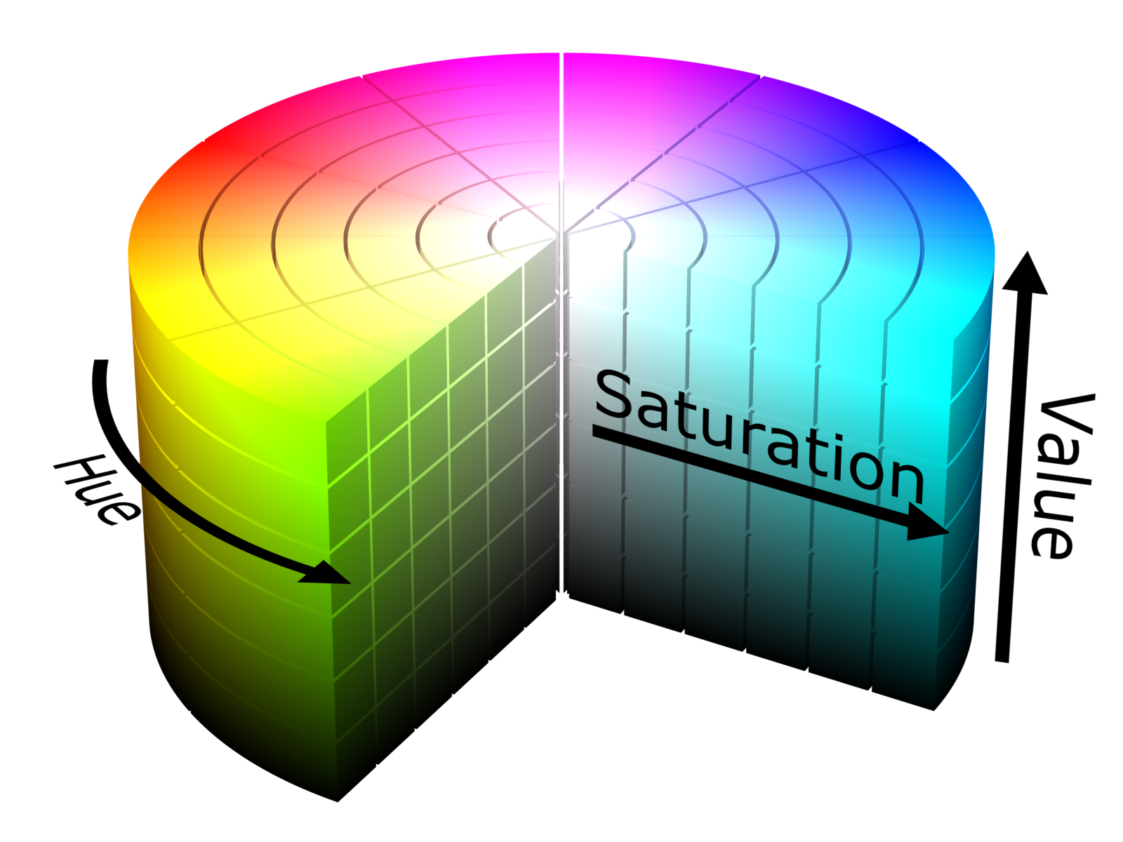
The HSV cylinder parts a rainbow of colours dispensed circularly
about its launch air top edge; hue refers to the angle along this
circle. The central axis of the cylinder ranges from black at the
bottom to white at the pause, with grey shades in between – this entire
axis has zero saturation, or intensity of color, and the gleaming hues
on the launch air circumference all have a saturation of 1.zero. In the end,
worth refers to the final brightness of the color, starting from
black at the bottom to intellectual shades at the pause.

So now let’s rethink our colours above, this time in the case of worth
and saturation:

Color	Fee	Saturation	Fee diff. from BG	Sat. diff from BG
white	zero.949	zero.017	—	—
grey	zero.659	zero.048	zero.290	zero.031
black	zero.286	zero.027	zero.663	zero.011
crimson	zero.859	zero.621	zero.090	zero.604
pink	zero.953	zero.263	zero.004	zero.247

As you might maybe maybe build an tell to, white, black, and grey differ deal in
worth, but part in the same method low saturation phases – successfully under
both crimson or pink. With the further knowledge supplied by HSV,
we can successfully label a pixel as belonging to the foreground if
both one in all these standards holds:

• the worth differs by extra than zero.Three from the background color, or
• the saturation differs by extra than zero.2 from the background color

The aged criterion pulls in the black pen marks, whereas the latter
pulls in the crimson ink as well to the pink line. Both standards
successfully exclude the grey bleed-through from the foreground.
Varied pictures will also require various saturation/worth thresholds;
seek the results part for facts.

As soon as we isolate the foreground, we’re left with a peculiar situation of colours
a lot just like the marks on the page. Let’s visualize the location – but
this time, as a replacement of pondering colours as a series of pixels, we
will preserve in thoughts them as 3D parts in the RGB colorspace. The resulting
scatterplot finally ends up taking a look rather “clumpy”, with several bands of
connected colours:

Our aim now might maybe be to transform the traditional 24 bit-per-pixel image into an
indexed color image by picking a tiny number (eight, on this case)
of colours to affirm the overall image. This has two effects: first,
it reduces the file size because specifying a color now requires simplest
Three bits (since ). Furthermore, it makes the resulting image
extra visually cohesive because in the same method colored ink marks are seemingly
to be assigned the equivalent color in the final output image.

To attain this aim we’re going to use an data-pushed method that
exploits the “clumpy” nature of the blueprint above. Deciding on colours
that correspond to the services of clusters will
consequence in a situation of colours that accurately represents the underlying
data. In technical terms, we’ll be fixing a color quantization
tell (which is itself true a determined case of
vector quantization), during the use of cluster diagnosis.

The explicit methodological instrument for the job that I picked is
k-method clustering. Its overall aim is to win a situation of
method or services which minimizes the life like distance from each and every level
to the nearest center. Here’s what you earn while you use it to purchase out
seven various clusters on the dataset above:

On this blueprint, the parts with black outlines convey foreground
color samples, and the colored lines join them to their closest
center in the RGB colorspace. When the image is remodeled to indexed
color, each and every foreground sample will earn modified with the color of the
closest center. In the end, the circular outlines masks the gap
from each and every center its furthest connected sample.

Other than being in a position to situation the worth and saturation thresholds, the
noteshrink.py program has several other principal parts. By
default, it will enhance the vividness and incompatibility of the final palette
by rescaling the minimal and maximum intensity values to zero and 255,
respectively. Without this adjustment, the eight-color palette for the
scan above would look hang this:

The adjusted palette is extra involving:

There will most seemingly be an technique to force the background color to white after
keeping apart the foreground colours. To additional lower the PNG image
sizes after conversion to indexed color, noteshrink.py can
robotically speed PNG optimization tools similar to optipng,
pngcrush, or pngquant.

The program’s final output combines several output pictures collectively
into PDFs hang this one the use of ImageMagick’s convert instrument. As a
additional bonus, noteshrink.py robotically kinds enter filenames
numerically (in exclaim of alphabetically, because the shell globbing
operator does). Here’s critical when your dumb scanning program
produces output filenames hang scan 9.png and scan 10.png, and likewise you
don’t prefer their lisp to be swapped in the PDF.

Here are some extra examples of the program output. The well-known one
(PDF) looks mammoth with the default
threshold settings:

Here is the visualization of the color clusters:

The subsequent one (PDF) required reducing
the saturation threshold to zero.045 since the blue-grey lines are so
drab:

Color clusters:

In the end, an instance scanned in from engineer’s graph paper
(PDF). For this one, I
situation the worth threshold to zero.05 since the incompatibility between the
background and the lines used to be so low:

Color clusters:

All collectively, the 4 PDFs settle up about 788KB, averaging about about
130KB per page of output.

I’m delighted I was in a position to contrivance a functional instrument that I will use to
put collectively scribe lisp PDFs for my route web sites. Previous that, I in fact
loved getting inspiring this writeup, especially since it prodded me to
strive to pork up on the undoubtedly 2D visualizations displayed on the
Wikipedia color quantization page, and likewise to in the raze learn
three.js (very fun, would use all once more).

If I ever revisit this project, I’d gain to debris round with
various quantization schemes. One which befell to me this week
used to be to utilize spectral clustering on the nearest neighbor graph of
a situation of color samples – I believed this used to be an exhilarating unusual thought after I
dreamed it up, but it turns on the market’s a 2012 paper that proposes this
real reach. Oh successfully.

You will also strive the use of expectation maximization to present a
Gaussian mixture mannequin describing the color distribution – no longer definite
if that’s been completed valuable in the previous. Varied fun suggestions comprise trying
out a “perceptually uniform” colorspace hang L*a*b* to cluster in, and
also to strive to robotically pick the
“finest” number of clusters for a given image.

On the opposite hand, I’ve obtained a backlog of blog entries to shove out the
door, so I’m going to construct a pin on this project for now, and invite you to head
checkout the noteshrink.py github repository. Until subsequent time!